Implementing an Autoencoder in TensorFlow 2.0
Posted by Senti AI
March 28, 2019

Google announced a major upgrade on the world’s most popular open-source machine learning library, TensorFlow, with a promise of focusing on simplicity and ease of use, eager execution, intuitive high-level APIs, and flexible model building on any platform.
This post is a humble attempt to contribute to the body of working TensorFlow 2.0 examples. Specifically, we shall discuss the subclassing APIimplementation of an autoencoder.
To install TensorFlow 2.0, it is recommended to create a virtual environment for it,
pip install tensorflow==2.0.0-alpha
or if you have a GPU in your system,
pip install tensorflow-gpu==2.0.0-alpha
More details on its installation through this guide from tensorflow.org.
Before diving into the code, let’s discuss first what an autoencoder is.
Autoencoder
We deal with huge amount of data in machine learning which naturally leads to more computations. However, we can also just pick the parts of the data that contribute the most to a model’s learning, thus leading to less computations. The process of choosing the important parts of the data is known as feature selection, which is among the number of use cases for an autoencoder.
But what exactly is an autoencoder? Well, let’s first recall that a neural network is a computational model that is used for finding a function describingthe relationship between data features x and its values (a regression task) or labels (a classification task) y, i.e. y = f(x).
Now, an autoencoder is also a neural network. But instead of finding the function mapping the features x to their corresponding values or labels y, it aims to find the function mapping the features x to itself x. Wait, what? Why would we do that?
Well, what’s interesting is what happens inside the autoencoder. Let’s bring up a graphical illustration of an autoencoder for an even better understanding.
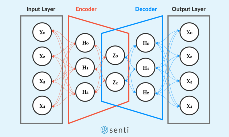
From the illustration above, an autoencoder consists of two components: (1) an encoder which learns the data representation, i.e. the important features zof the data, and (2) a decoder which reconstructs the data based on its idea zof how it is structured.
Going back, we established that an autoencoder wants to find the function that maps x to x. It does so through its components. Mathematically,


The encoder h-sub-e learns the data representation z from the input features x, then the said representation serves as the input to the decoder h-sub-d in order to reconstruct the original data x.
We shall further dissect this model below.
Encoder
The first component, the encoder, is similar to a conventional feed-forward network. However, it is not tasked on predicting values or labels. Instead, it is tasked to learn how the data is structured, i.e. data representation z.
The encoding is done by passing data input x to the encoder’s hidden layer h in order to learn the data representation z = f(h(x)). We can implement the Encoder layer as follows,
We first define an Encoderclass that inherits the tf.keras.layers.Layer to define it as a layer instead of a model. Why a layer instead of a model? Recall that the encoder is a component of the autoencoder model.
Going through the code, the Encoder layer is defined to have a single hidden layer of neurons (self.hidden_layer) to learn the activation of the input features. Then, we connect the hidden layer to a layer (self.output_layer) that encodes the data representation to a lower dimension, which consists of what it thinks as important features. Hence, the “output” of the Encoder layer is the learned data representation z for the input data x.
Decoder
The second component, the decoder, is also similar to a feed-forward network. However, instead of reducing data to a lower dimension, it reconstructs the data from its lower dimension representation z to its original dimension x.
The decoding is done by passing the lower dimension representation z to the decoder’s hidden layer h in order to reconstruct the data to its original dimension x = f(h(z)). We can implement the decoder layer as follows,
We define a Decoderclass that also inherits the tf.keras.layers.Layer.
The Decoder layer is also defined to have a single hidden layer of neurons to reconstruct the input features from the learned representation by the encoder. Then, we connect its hidden layer to a layer that decodes the data representation from a lower dimension to its original dimension. Hence, the “output” of the decoder layer is the reconstructed data x from the data representation z. Ultimately, the output of the decoder is the autoencoder’s output.
Now that we have defined the components of our autoencoder, we can finally build the model.
Building the Autoencoder model
We can now build the autoencoder model by instantiating the Encoder and the Decoder layers.
As we discussed above, we use the output of the encoder layer as the input to the decoder layer. So, that’s it? No, not exactly.
To this point, we have only discussed the components of an autoencoder and how to build it, but we have not yet talked about how it actually learns. All we know to this point is the flow of data; from the input layer to the encoder layer which learns the data representation, and use that representation as input to the decoder layer that reconstructs the original data.
Like other neural networks, an autoencoder learns through backpropagation. However, instead of comparing the values or labels of the model, we compare the reconstructed data x-hat and the original data x. Let’s call this comparison the reconstruction error function, and it is given by the following equation,

The reconstruction error in this case is the function that you're likely to be familiar with
In TensorFlow, the above equation could be expressed as follows,
Are we there yet? Close enough. Just a few more things to add. Now that we have our error function defined, we can finally write the training function for our model.
This way of implementing backpropagation affords us with more freedom by enabling us to keep track of the gradients, and the application of an optimization algorithm to them.
Are we done now? Let’s see.
- Define an encoder layer. Checked.
- Define a decoder layer. Checked.
- Build the autoencoder using the encoder and decoder layers. Checked.
- Define the reconstruction error function. Checked.
- Define the training function. Checked.
Yes! We’re done here! We can finally train our model!
But before doing so, let’s instantiate an Autoencoder class that we defined before, and an optimization algorithm to use. Then, let’s load the data we want to reconstruct. For this post, let’s use the unforgettable MNIST handwritten digit dataset.
We can visualize our training results by using TensorBoard, and to do so, we need to define a summary file writer for the results by using tf.summary.create_file_writer.
Next, we use the defined summary file writer, and record the training summaries using tf.summary.record_if.
We can finally (for real now) train our model by feeding it with mini-batches of data, and compute its loss and gradients per iteration through our previously-defined train function, which accepts the defined error function, the autoencoder model, the optimization algorithm, and the mini-batch of data.
After each iteration of training the model, the computed reconstruction error should be decreasing to see if it the model is actually learning (just like in other neural networks). Lastly, to record the training summaries in TensorBoard, we use the tf.summary.scalar for recording the reconstruction error values, and the tf.summary.image for recording the mini-batch of the original data and reconstructed data.
After some epochs, we can start to see a relatively good reconstruction of the MNIST images.

Results on MNIST handwritten digit dataset. Images at the top row are the original ones while images at the bottom row are the reconstructed ones.
The reconstructed images might be good enough but they are quite blurry. A number of things could be done to improve this result, e.g. adding more layers and/or neurons, or using a convolutional neural network architecture as the basis of the autoencoder model, or use a different kind of autoencoder.
Closing remarks
Autoencoders are quite useful for dimensionality reduction. But it could also be used for data denoising, and for learning the distribution of a dataset. I hope we have covered enough in this article to make you excited to learn more about autoencoders!
References
- Martín Abadi, Ashish Agarwal, Paul Barham, Eugene Brevdo, Zhifeng Chen, Craig Citro, Greg S. Corrado, Andy Davis, Jeffrey Dean, Matthieu Devin, Sanjay Ghemawat, Ian Goodfellow, Andrew Harp, Geoffrey Irving, Michael Isard, Rafal Jozefowicz, Yangqing Jia, Lukasz Kaiser, Manjunath Kudlur, Josh Levenberg, Dan Mané, Mike Schuster, Rajat Monga, Sherry Moore, Derek Murray, Chris Olah, Jonathon Shlens, Benoit Steiner, Ilya Sutskever, Kunal Talwar, Paul Tucker, Vincent Vanhoucke, Vijay Vasudevan, Fernanda Viégas, Oriol Vinyals, Pete Warden, Martin Wattenberg, Martin Wicke, Yuan Yu, and Xiaoqiang Zheng. TensorFlow: Large-scale machine learning on heterogeneous systems,
2015. Software available from tensorflow.org. - Chollet, F. (2016, May 14). Building Autoencoders in Keras. Retrieved March 19, 2019, from https://blog.keras.io/building-autoencoders-in-keras.html
- Goodfellow, I., Bengio, Y., & Courville, A. (2016). Deep learning. MIT press.
Want to know more?
More Resources you may like

AI in Healthcare: Research, Applications, and Challenges

Mayor Isko Uses Artificial Intelligence for City of Manila

